Measuring Displacements Using Accelerometers: Part 2- Comparing Methods and Integration

In the last post I discussed the methods I looked into for cancelling the gravity vectors measured by the ACC, if you haven’t seen that I would recommend reading that first. The way I compared the two methods was by seeing how well they follow the raw acceleration signal from an angular movement, this was done by mounting the sensor on the side of a servo motor and moving between different angles with varying starting positions(in reference to gravity) and magnitudes of angle change. Below is the graph from a 5-degree movement.

The blue graph is the raw acceleration signal on the Z axis,red is the cos method and the yellow is the tan method, looking at the full graph(left picture) they seem to be overlapped and looks like they both follow the raw signal fairly well but in the zoomed in picture(right), both are slightly off the middle of the raw acceleration so neither seems better than the other, the Y axis showed the same result that neither stood out. I did another test where the angle change was 35 degrees and the result of the of the two axes is below:

In these two graphs its a lot more obvious which is the more accurate, the tan method fails at following the movement for this magnitude of angle change, the cos and sin method follows but not to the accuracy I’d hope. The drift seen after the during the pause is caused by the gyroscopes drift rather than the vector equations, the gyroscope is accurate for small angle changes but the bigger the angle change the further the angle measured is from the real value and the more it drifts when stationary. And as I mentioned before in the previous post this application won’t have angle changes larger than around 5 degrees so the gyroscope error won’t be as noticeable. Even though both were accurate for the 5-degree change, I decided to go with the cos sin method because it seems more mathematically sound from the results of the last test. At this point when I was working on this I thought “Ah now I just have to integrate the movement acceleration twice and I’ll have my displacement” but this wasn’t true, getting the actual displacement from the acceleration took me a lot longer than I hoped it would but I did get it in the end, just encase you thought reading this was going to waste your time, but now I’m going to talk about the integration, the problems I had and the workarounds I had to use to get it working.

Integration

As I mentioned in the previous post we need to integrate the output of the gyroscope to give us the angle and I’m going to go through that first before the acceleration. The integration of the gyroscope can be written as follows

This basically says the angle at sample n is the sum of the previous angles plus the current angular velocity multiplied by the sample interval, this can be written in code as

Y(n)=Y(n-1)+X(n)*Ts

Y being the output(angle) and X being the input(angular velocity) and if the discrete transfer function of this formula is found and graphed, you can see that integration works as a low-pass filter with a gain of -20dB/decade and for the case of the acceleration, as it’s integrated twice, the gain is -40dB/decade and this produces a smooth output free of any high-frequency signals. Below are the raw gyroscope output and the integrated angle from a 5-degree angle change.

So in the angle graph you can see that it has gotten rid of the noise from the raw data showing the low-pass filtering effect from the integration working, other than the integration, the only other thing done to the raw data was removing the DC offset. Below shows the same method for double integrating double integrating the acceleration.

This is from a linear/angular movement of a few millimetres which the starting and ending position is the same but the displacement graph doesn’t reflect this, it just shows  a displacement which moves backwards and then shoots forward and never returns so this graph is definitely incorrect. This was a problem I was facing for a long time on how to get the correct displacement from a movement which included both angular and  linear motions, I tried many different methods, wrote lots of different codes but after a while I found a way that would get the shape and magnitude of the displacement expected but it required me to make an assumption about the movement I was measuring. Even though the calculations used for removing gravity worked fairly well, there would sometimes still be a tiny offset from zero and this would cause the first integrated graph(velocity) to ramp up where the velocity should be zero and once the actual movement gets integrated, it’s hidden under the ramp created by the error, this ramp once integrated , it turns into half of a parabola-like shape, like the displacement graph above. So the assumption to get rid of this error was that the starting and ending position so the mean of the acceleration should be zero. So after the calculated gravity is removed, the mean of the whole set of data is calculated and subtracted so that the data is zeroed. This did improve the displacement graph but still wasn’t perfect because integrating the parts of the graph where no movement was present was causing problems, so the way around this was to let the user choose which the parts of the graph get integrated so that the error caused by integration is reduced. Using both of these methods is what finally got displacements which had the shape and magnitude that was expected. The graph below is the displacement from the previous acceleration using this new method.

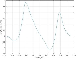
This seems a lot more plausible than the previous graph as the expected magnitude of the displacement was a few millimetres and the shape was expected to have the same starting and ending position. In the next post, I’m going to go into more detail about the testing and have a video showing it measuring a linear movement.

<< Part 1 – Part 3 >>